How To Create Donut Chart In Excel

Home / Charts / Excel Doughnut Chart to Measure Progress to a Goal

An Excel Doughnut chart is a very popular way to measure progress towards a goal or target. They are simple to understand, appealing to the eye and familiar to users.

You see Doughnut charts being used to show progress in the news, in business reports and even when your computer is loading or refreshing.

Well the good news is that they are also extremely easy to create.

Watch the Video

Set up the Data

You will probably have a percentage in a cell on your spreadsheet showing your progress toward the goal. This is probably the result of some formula in a 'real world' situation.

For this example we have just typed a percentage into cell B2.

You will need to calculate the remaining percentage in another cell. You can do this by typing the following formula.

=1-B2

This formula subtracts the progress percentage from 1 to return the remaining percentage.

Create the Excel Doughnut Chart

With these values we can now create the Doughnut chart.

Select the two values (range B2:B3 in this example).
Click the Insert tab, Pie chart button and select the Doughnut chart (the location of the Doughnut chart button may differ on your Excel version).

And as easy as that, you have a Doughnut chart in Excel showing progress.

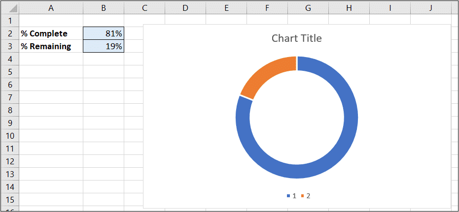
Basic Excel Doughnut chart showing progress complete

It is however a little basic, so lets do some formatting to bring it to life.

Format the Doughnut Chart to Make it Amazing

We will now apply some formatting steps to bring our Doughnut chart up a level.

Click on the Chart Title placeholder and type a meaningful title.
Click on the Legend (completely redundant in this situation) and press Delete on the keyboard to remove it.
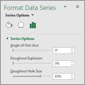
Double click on the Doughnut Chart itself (on the data series) and this should open the Data Series task pane (shown below Excel 2016, your version may open a dialog box). Adjust the Doughnut Hole Size to 65%.

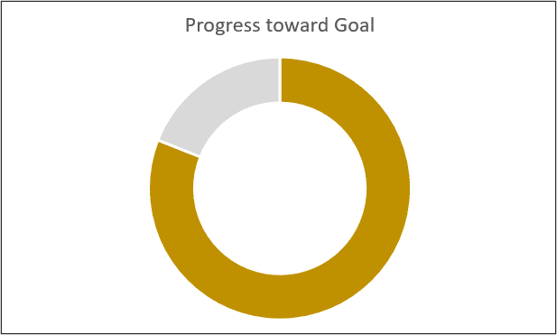
Click on the data point for the remaining percentage, click the Format tab, and select a light colour from the Shape Fill list. I chose a light grey.
Then click the data point for the progress percentage and select a brighter and more vibrant colour to catch the reader focus from the Shape Fill list on the Format tab. I chose a Gold colour.

The chart will now look like below. A big improvement. Our final step will be to add the big percentage value into the hole of the doughnut.

Improved Excel Doughnut chart showing progress toward a goal

Add a Text Box for the Percentage Value

Click the Insert tab and then the Text box button.
Click and drag to draw the text box into position. This does not need to be accurate, as it can be moved and resized later.
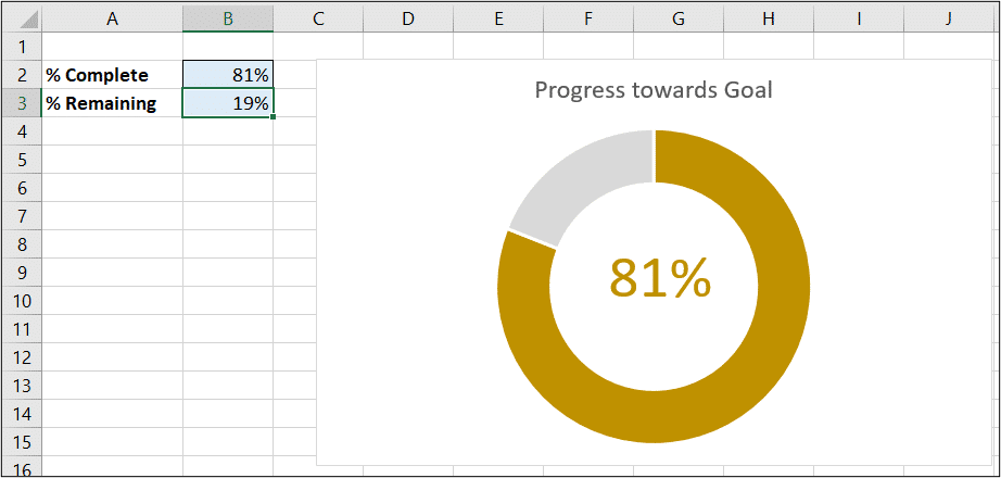
With the text box selected, click in the Formula bar, type =B2 (or whatever cell your progress percentage is in) and press Enter.
You can then format the text how you wish. I made the font size 32, the same Gold colour as the chart progress and also bold.

Completed chart with progress percentage

Reader Interactions